Updated September 17, 2026. Added filtered retrieval evaluation and an eligible-corpus baseline, extending the series beyond unfiltered nearest-neighbor examples.
Retrieval quality has a sweet spot. Both extremes hurt; the curve depends on your queries, corpus, and embedding model.
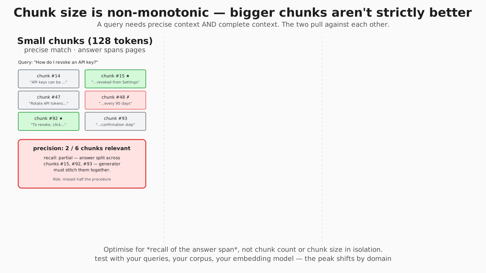
Chunk size is non-monotonic — bigger chunks aren't strictly better
Building On Previous Knowledge
The previous chapter showed that LLMs generate token-by-token from a learned probability distribution — and crucially, even with temperature = 0 and a fixed seed, generation isn’t bit-identical across hardware. That non-determinism is the second-order problem. The first-order one is more obvious: the model can only generate from patterns it memorised during training. New facts, your private data, this week’s news — none of it is in there.
If the answer isn’t in the training data, the model refuses to answer or, worse, fabricates a plausible-sounding response.
Where most RAG tutorials stop: they tell you to “chunk your documents”, “embed them”, “query the vector store”, and ship. They never explain why chunk-size 128 fragments answers across pages, why chunk-size 2048 triggers Lost-in-the-Middle, why dense retrieval misses exact strings like E1234, or why BM25 — a 1994 algorithm — still beats fancy embeddings on keyword-heavy queries. This chapter walks the data path through Karpukhin et al. 2020 (DPR) [karpukhin2020], Robertson & Zaragoza’s BM25 [robertson2009], and Chroma’s 2025 Context Rot measurements [chroma-rot]. Every claim has a number you can verify.
Takeaway: retrieval grounds generation in facts the model never saw — but the configuration choices (chunk size, sparse vs dense, single-stage vs reranked) determine whether the grounding is precise enough to matter.
What Goes Wrong Without This:
Symptom: Your AI assistant confidently answers questions about your
       company's products with completely fabricated information.
Cause:   The LLM generates plausible text from patterns, but has no
       access to your actual documentation. High confidence ≠ correctness.

Symptom: Retrieval returns documents with high similarity scores,
but the RAG system still produces incorrect answers.
Cause: You treated retrieval as similarity search. Similarity is
SYMMETRIC (A similar to B = B similar to A). Relevance is NOT.

Symptom: RAG works for demo queries but fails for real user queries.
Cause: Demo queries match document phrasing. Real queries use
different vocabulary. Query-document mismatch.
The Limits of Pure Generation
LLMs are trained on static data with a cutoff date. They generate from learned patterns, not live facts.
Problems with pure generation:

1. KNOWLEDGE CUTOFF
 Q: "Who won the 2024 election?"
 A: "I don't have information past my training cutoff..."

2. HALLUCINATION
 Q: "What's the API for uploading files in our product?"
 A: "Use POST /api/upload with multipart/form-data..."
 (confidently wrong—made up based on patterns)

3. NO PRIVATE DATA
 Q: "What did the client say in yesterday's email?"
 A: Cannot access—not in training data

4. OUTDATED FACTS
 Q: "What's the current price of Bitcoin?"
 A: Training data price, not live price
The model generates plausible text, but plausible ≠ true.
Takeaway: every LLM has a knowledge cutoff, hallucinates confidently on facts it doesn’t have, and cannot read your private data — three failure modes that no amount of bigger-model scaling will fix without external context.
Retrieval: Grounding Generation in Facts
Instead of asking the model to recall facts, give it facts to use.
Without retrieval:
User query → LLM → Generated answer (may hallucinate)

With retrieval:
User query → Search knowledge base → Relevant docs
↓
[Query + Docs] → LLM → Grounded answer

The LLM now has context to work with.
The Retrieval Pipeline
INDEXING (offline):

Documents
│
↓
┌───────────┐
│ Chunk │ Split into manageable pieces
└───────────┘
│
↓
┌───────────┐
│ Embed │ Convert chunks to vectors
└───────────┘
│
↓
┌───────────┐
│ Index │ Store in vector database
└───────────┘

QUERY (online):

User query
│
↓
┌───────────┐
│ Embed │ Same embedding model as indexing
└───────────┘
│
↓
┌───────────┐
│ Search │ Find similar vectors in index
└───────────┘
│
↓
Top-K most similar chunks
Vector Similarity Search
Core mechanic: find vectors closest to query vector.
Query embedding: [0.2, 0.8, -0.1, ...]

Document embeddings in index:
doc1: [0.25, 0.75, -0.05, ...] → sim = 0.98 ← most similar
doc2: [0.1, 0.6, 0.3, ...] → sim = 0.85
doc3: [-0.5, 0.1, 0.8, ...] → sim = 0.23
doc4: [0.22, 0.78, -0.08, ...] → sim = 0.97

Return top-K (e.g., K=3): [doc1, doc4, doc2]
Why it works: Embedding models map similar meanings to similar vectors. “How do I reset my password?” is close to “Password reset instructions” even though they share few words.
Takeaway: retrieval factors generation into two stages — find relevant context offline-indexed, generate against it online — so the model becomes a reading-comprehension engine over text it has just been shown, not a memory engine over text it once saw.
Dense vs Sparse Retrieval
Two fundamentally different approaches:
SPARSE RETRIEVAL (BM25, TF-IDF):
Representation: High-dimensional sparse vectors
(vocab_size dimensions, mostly zeros)

"The cat sat" → [0, 0, ..., 1, 0, ..., 1, 0, ..., 1, ...]
↑ ↑ ↑
cat sat the

Matching: Exact keyword overlap
Strengths: Precise keyword matching, interpretable
Weakness: Misses synonyms, requires exact terms

DENSE RETRIEVAL (Embeddings):
Representation: Low-dimensional dense vectors
(384-1536 dimensions, all non-zero)

"The cat sat" → [0.23, -0.41, 0.89, 0.12, ...]

Matching: Semantic similarity
Strengths: Captures meaning, handles synonyms
Weakness: May miss exact matches, less interpretable
The dense vs sparse contest isn’t settled. Karpukhin et al. 2020’s Dense Passage Retrieval paper showed dense retrievers outperform “a strong Lucene-BM25 system largely by 9%–19% absolute in terms of top-20 passage retrieval accuracy” on open-domain QA [karpukhin2020] — but that’s on natural-language questions paired with Wikipedia passages. Flip the workload to keyword-heavy queries (“error code E1234”, “stack trace NullPointerException”) and BM25 wins. The canonical BM25 formula (Robertson & Zaragoza 2009 [robertson2009]) uses two parameters — k₁ controls term-frequency saturation, b controls document-length normalisation. Lucene ships k₁ = 1.2, b = 0.75 by default; the literature recommends tuning k₁ within [1.2, 2.0]. Don’t tune them until you’ve measured.
In practice: Combine both (hybrid search).
Query: "error code E1234"

Sparse (BM25): Finds docs with exact string "E1234" ✓
Dense: May not find if "E1234" wasn't in training data ✗

Query: "my application keeps crashing"

Sparse (BM25): Needs exact word "crashing" ✗
Dense: Matches "app failure", "program stops working" ✓

Hybrid: Best of both
Reciprocal Rank Fusion (RRF)
When combining dense and sparse results, use RRF to merge ranked lists:
RRF_score(doc) = Σ 1 / (k + rank_i(doc))

Where:

- rank_i(doc) = position of doc in ranking i (1-indexed)
- k = constant (typically 60)

Example:
Dense ranking: [doc_A (rank 1), doc_B (rank 2), doc_C (rank 3)]
Sparse ranking: [doc_B (rank 1), doc_C (rank 2), doc_A (rank 3)]

RRF scores (k=60):
doc_A: 1/(60+1) + 1/(60+3) = 0.0164 + 0.0159 = 0.0323
doc_B: 1/(60+2) + 1/(60+1) = 0.0161 + 0.0164 = 0.0325 ← Highest!
doc_C: 1/(60+3) + 1/(60+2) = 0.0159 + 0.0161 = 0.0320

Final ranking: [doc_B, doc_A, doc_C]
RRF is simple and often performs just as well as learned score combination — Cormack, Clarke, Buettcher 2009 published the original k=60 default and the SIGIR evaluation showing it outperforms Condorcet and learned rank-aggregation methods [cormack2009].
Takeaway: dense retrieval wins on natural-language questions (DPR’s 9–19% lead on open-domain QA); sparse BM25 wins on keyword-heavy or out-of-distribution queries. Hybrid + RRF gets you both with one configuration knob (k=60) and no learned model.
Chunking: Why and How
Documents are too long to embed as single units:
- Embedding models have token limits (512-8192)
- Long texts dilute specific information
- Retrieval granularity matters
Document: 50-page manual

Bad: One embedding for entire document
→ Query matches but relevant info buried in noise

Good: Chunk into ~500 token pieces
→ Query matches specific relevant section
Chunking Strategies
Fixed-size: Every N tokens
Simple, may break mid-sentence

Sentence-based: Split at sentence boundaries
Preserves complete thoughts

Paragraph-based: Split at paragraph breaks
Preserves larger context

Semantic: Split where topic changes
Best quality, more complex

Recursive: Try larger splitters first, fall back
Hierarchical, respects structure
Overlap
Include some text from previous chunk to preserve context at boundaries:
Chunk 1: "...the password reset link. Click it to..."
Chunk 2: "...reset link. Click it to create a new password..."
                  ↑
            overlap region

Why: Context at boundaries isn't lost.
Tradeoff: More storage, potential duplicate retrieval.
Why Chunk-Size Is Non-Monotonic
This is the chapter’s load-bearing claim, and the one that most public RAG tutorials skip: bigger chunks are not strictly better. The recall-vs-chunk-size curve has an interior maximum, not a monotonic shape. The hero diagram shows the curve qualitatively; the mechanism is the tension between two effects:
- Too small (e.g. 128 tokens) → the answer fragments across multiple chunks. The retriever returns chunk #15 (“revoked from Settings”) but misses chunk #92 (“click confirm”). The generator now has half the procedure. Recall is partial of the answer span, even though the chunks “matched” the query.
- Too large (e.g. 2048 tokens) → each chunk contains the answer and 1,500 tokens of unrelated context. Two compounding harms: (1) dense-embedding precision drops because one vector now represents many topics; (2) Lost-in-the-Middle kicks in at generation time. Liu et al. 2023 named the U-shaped attention-vs-position pattern [liu2023]. Chroma’s 2025 Context Rot report then tested 18 LLMs across Anthropic, OpenAI, Google, and Alibaba and found “performance grows increasingly unreliable as input length grows”, with target information at the start outperforming target information in the middle [chroma-rot].
The Chroma study added a counter-intuitive finding: “models perform worse when the haystack preserves a logical flow of ideas. Shuffling the haystack and removing local coherence consistently improves performance” across all 18 models tested [chroma-rot]. Coherent long chunks aren’t free — coherence itself becomes a distractor.
The peak commonly lands around 256–512 tokens for English natural-language corpora with a text-embedding-3-small-class model — the peak shifts with embedding model, corpus structure, and query type. Test, don’t guess.
Takeaway: chunk size has an interior optimum, not a monotonic curve. Both 128-token fragmentation and 2048-token Lost-in-the-Middle hurt recall — usually peak at 256–512 tokens for English NL queries, but measure on your corpus.
Multi-Stage Retrieval
Single-stage retrieval trades off speed vs accuracy. Multi-stage gets both.
SINGLE-STAGE RETRIEVAL
--------------------------------------------------------------------

Query → Embedding Model → Vector Search → Top 10 Results

Fast (~20ms), but accuracy limited by bi-encoder's ability
to independently embed query and docs.

MULTI-STAGE RETRIEVAL (Retrieve → Rerank)
──────────────────────────────────────────

Stage 1: Fast retrieval (bi-encoder)
Query → Top 100 candidates (~20ms)
Uses: Dense/sparse/hybrid retrieval

Stage 2: Accurate reranking (cross-encoder)
Rerank 100 → Top 10 (~200ms for 100 pairs)
Uses: Cross-encoder model

Total: ~250ms, but significantly better accuracy
Bi-Encoder vs Cross-Encoder
BI-ENCODER (used in retrieval):

Query ─────→ [Encoder] ─────→ query_vector
↓
cosine_similarity = score
↑
Doc ─────→ [Encoder] ─────→ doc_vector

✓ Can pre-compute doc vectors (once)
✓ Fast similarity search at query time
✓ Scales to millions of documents
✗ Query and doc don't "see" each other
✗ Lower accuracy

CROSS-ENCODER (used in reranking):

[CLS] query [SEP] document [SEP] ─────→ [BERT] ─────→ score

✓ Query and doc interact via attention
✓ Higher accuracy (5-10% improvement)
✗ Must encode every (query, doc) pair
✗ Can't pre-compute anything
✗ Slow: O(n) for n documents
Why Two Stages?
┌──────────────────────────┬───────────┬──────────┬───────────────────┐
│ Method                   │ Latency   │ Accuracy │ Use Case          │
├──────────────────────────┼───────────┼──────────┼───────────────────┤
│ Bi-encoder only          │ ~20ms     │ 85%      │ Speed-critical    │
│ Cross-encoder only       │ ~20s/1M   │ 95%      │ Tiny corpus only  │
│ Bi-encoder → Cross-enc   │ ~250ms    │ 93%      │ Production        │
└──────────────────────────┴───────────┴──────────┴───────────────────┘

The bi-encoder filters to candidates.
The cross-encoder reranks for precision.
Best of both worlds.
Takeaway: single-stage retrieval is bound by the bi-encoder’s ability to embed query and doc independently; multi-stage adds a cross-encoder reranker that lets the query and doc attend to each other — typical 5–10pp accuracy gain for ~10× latency in the reranking pass.
Retrieval Quality Metrics
How do you know retrieval is working?
Recall@K
"Of all relevant docs, how many are in my top-K?"

5 relevant docs exist, top-10 retrieval finds 4
Recall@10 = 4/5 = 0.80

Critical for RAG: if relevant doc isn't retrieved,
the LLM can't use it.

Precision@K
"Of my top-K results, how many are relevant?"

Top-10 has 4 relevant, 6 irrelevant
Precision@10 = 4/10 = 0.40

Matters for: context window efficiency, noise reduction

MRR (Mean Reciprocal Rank)
"How high is the first relevant result?"

First relevant at position 3 → RR = 1/3
Average across queries = MRR
For RAG, Recall@K usually matters most. If the answer isn’t retrieved, generation fails.
Takeaway: Recall@K is the primary metric for RAG — if the answer span isn’t in the top-K, no generator can recover. Precision@K and MRR matter for cost and UX; Recall@K matters for correctness.
Common Pitfalls & Misconceptions
The table below names the failure modes that show up most often in production RAG. Each row is a concrete bug class — the subsections that follow expand the trickiest three.
| Symptom | Cause | Fix |
|---|---|---|
| Similarity scores are high but answers are still wrong | Similarity is symmetric; relevance is not. A doc that matches the query may still not answer it (“How do I bake cookies?” vs “I baked cookies yesterday”). | Rerank with a cross-encoder; evaluate Recall@K against held-out answer spans, not blind similarity thresholds. |
| RAG works on demo queries, fails on real user queries | Query-document phrasing mismatch — demo queries echo the docs; real users use synonyms (“login bug” vs “authentication failure”). | Add HyDE (generate hypothetical answer, embed that), query rewriting, or fine-tune the retriever on real (query, doc) pairs from your domain. |
| Retrieval “succeeds” but generator produces wrong answer | Answer is split across two chunks; neither alone is sufficient. Each chunk scores medium similarity, generator gets fragments. | Increase chunk overlap (15–25% of chunk size is a common default), or move to a coarser chunk size — then re-measure Recall@K of the answer span, not chunks. |
| Top-K chunks all match the query but bury the answer | Chunk size too large; Lost-in-the-Middle hides the answer span inside ~2K tokens of noise (Chroma 2025 measured this across 18 LLMs). | Reduce chunk size to 256–512 tokens, or post-process retrieved chunks (sentence-window retrieval) so the generator sees a tight passage, not a 2KB block. |
| Dense retrieval misses exact error codes | Dense embeddings smear rare tokens (E1234, NullPointerException) into nearby semantic space; they don’t preserve exact strings the way BM25 does. | Use hybrid (BM25 + dense) with RRF combination. BM25 anchors the exact-match path; dense handles paraphrase. |
| Embedding model upgrade silently breaks production | Different embedding models produce different vector spaces — old indexed chunks aren’t comparable to new query embeddings. | Re-index the entire corpus when changing embedding models. Treat the embedding model as part of the index schema, not a swappable config flag. |
| Chunks hit the embedding model’s token limit and silently truncate | Embedding models cap at 512–8192 tokens; longer inputs are truncated server-side without warning. | Pin chunk size below the embedding model’s max_input_tokens (e.g. 8191 for text-embedding-3-large). Assert chunk-token-count at index time. |
Takeaway: RAG bugs almost always trace to one of these seven classes — and most look like “the model is bad” until you instrument retrieval separately from generation.
Misconception: “High similarity score = relevant result”
Query: "How do I bake cookies?"
Document: "I baked cookies yesterday and they were delicious."

Similarity: HIGH (same topic, same words)
Relevance: ZERO (describes past event, doesn't answer the question)

Similarity is SYMMETRIC. Relevance is NOT.
A relevant document must be similar, but a similar document
isn't necessarily relevant.
The Query-Document Mismatch Problem
Query:  "How do I fix the login bug?"
      (question format, user language)

Doc: "Authentication failures can be resolved by..."
(statement format, technical language)

Problem: Different phrasing may have lower similarity
even when doc answers the query.
Solutions:
- Query Expansion: Add synonyms and related terms
- HyDE: Generate hypothetical answer, embed that instead
- Query Rewriting: Transform user query to match document style
- Fine-tuned Retrievers: Train on your domain’s (query, doc) pairs
Chunking Mistakes
The correct answer might be split across two chunks.
Neither chunk alone answers the query.
Both chunks score medium similarity.
Retrieval "succeeds" (returns chunks).
RAG fails (no chunk contains the answer).

Chunking is a system design decision, not preprocessing trivia.
Code Example
A minimal hybrid (BM25 + dense) retriever in ~40 lines, pinned to current library versions. Uses sentence-transformers [sbert] for the dense path and rank-bm25 [rank-bm25] for the sparse path:
# Tested on:
#   sentence-transformers==3.0.1
#   rank-bm25==0.2.2
#   numpy==1.26.4
# Python 3.11
import numpy as np
from sentence_transformers import SentenceTransformer
from rank_bm25 import BM25Okapi

# 1. Corpus -------------------------------------------------------------------
documents = [
    "To reset your password, go to Settings > Security > Reset Password.",
    "Our API rate limit is 100 requests per minute for free tier.",
    "Authentication failures (error code E1234) require a password reset.",
    "Contact support@example.com for billing questions.",
    "The application requires Python 3.9 or higher.",
    "Two-factor authentication can be enabled in Settings > Security.",
]

# 2. Dense index (bi-encoder, normalized embeddings → dot = cosine) -----------
dense_model = SentenceTransformer("all-MiniLM-L6-v2")
dense_index = dense_model.encode(documents, normalize_embeddings=True)

# 3. Sparse index (BM25 with default k1=1.5, b=0.75) --------------------------
tokenised = [d.lower().split() for d in documents]
sparse_index = BM25Okapi(tokenised)  # rank-bm25 defaults: k1=1.5, b=0.75


def rrf_combine(rankings: list[list[int]], k: int = 60) -> list[int]:
    """Reciprocal Rank Fusion — Cormack et al. 2009. k=60 is the Lucene default."""
    scores: dict[int, float] = {}
    for ranking in rankings:
        for rank, doc_id in enumerate(ranking, start=1):
            scores[doc_id] = scores.get(doc_id, 0.0) + 1.0 / (k + rank)
    return sorted(scores, key=scores.get, reverse=True)


def hybrid_search(query: str, top_k: int = 3) -> list[tuple[str, float]]:
    q_dense = dense_model.encode(query, normalize_embeddings=True)
    dense_rank = np.argsort(dense_index @ q_dense)[::-1].tolist()

    sparse_rank = np.argsort(sparse_index.get_scores(query.lower().split()))[::-1].tolist()

    fused = rrf_combine([dense_rank, sparse_rank])[:top_k]
    return [(documents[i], float(dense_index[i] @ q_dense)) for i in fused]


for q in [
    "How do I change my password?",      # paraphrase — dense should win
    "error code E1234",                  # exact match — BM25 should win
    "I need help with my bill",          # paraphrase
]:
    print(f"\nQuery: {q!r}")
    for doc, score in hybrid_search(q, top_k=2):
        print(f"  [{score:.3f}] {doc[:60]}")
The hybrid result outperforms either retriever alone on a corpus this small — and the gap widens with bigger corpora and more varied queries. The “exact code E1234” query is the decisive test: pure dense often misses it; pure BM25 catches it; RRF gets both paths.
Verify Your Understanding
Before continuing, you should be able to answer these from memory:
- Similarity ≠ relevance, with a concrete example. Pick a query whose top-similarity doc is irrelevant. Explain in one sentence why similarity is symmetric and relevance is not.
- The Doc1 vs Doc2 trap. Query
"How do I reset my password?"— Doc1"Password reset failed for user X at 3:42pm"(sim=0.91) vs Doc2"Go to Settings > Security > Reset Password"(sim=0.87). Which is more relevant? Name the mechanism that lets cosine put the wrong doc on top. - “BM25 is outdated, dense retrieval is always better.” Identify the error. Cite a concrete query class where BM25 wins and explain why (hint: rare exact strings, OOV vocabulary).
- Recall@10 vs Precision@10. Retrieval returns 10 docs; 8 score high similarity, only 2 actually answer the question. Which metric exposes this failure? What does the other metric tell you instead?
- Walk through the chunk-size curve. At chunk size 128 you get fragmented answers; at 2048 you get Lost-in-the-Middle. Name the two opposing forces and predict where the peak lands for an English natural-language corpus on
text-embedding-3-small.
What’s Next
Retrieval gave us relevant chunks. The next chapter — Retrieval → RAG — wires those chunks into a generation prompt, covers prompt construction and reranking strategies, and walks the debugging decision tree: when retrieval is wrong vs when generation is wrong, and why most teams misdiagnose the failure.
References
- [karpukhin2020] Karpukhin, V. et al. Dense Passage Retrieval for Open-Domain Question Answering. EMNLP 2020. arXiv:2004.04906. Source for the 9–19% top-20 retrieval-accuracy gain of DPR over Lucene-BM25 on open-domain QA. Cited in §§ Building On Previous Knowledge, Dense vs Sparse Retrieval.
- [robertson2009] Robertson, S., Zaragoza, H. The Probabilistic Relevance Framework: BM25 and Beyond. Foundations and Trends in Information Retrieval, 2009. Canonical BM25 reference; covers the
k₁, bparameters and the term-frequency saturation argument. Cited in § Dense vs Sparse Retrieval. - [chroma-rot] Hong, K., Troynikov, A., Huber, J. Context Rot: How Increasing Input Tokens Impacts LLM Performance. Chroma Technical Report, 2025-07-14. trychroma.com/research/context-rot. Measured retrieval degradation across 18 LLMs as input length grew: Anthropic (Claude Opus 4, Sonnet 4, Sonnet 3.7, Sonnet 3.5, Haiku 3.5), OpenAI (o3, GPT-4.1, GPT-4.1 mini, GPT-4.1 nano, GPT-4o, GPT-4 Turbo, GPT-3.5 Turbo), Google (Gemini 2.5 Pro, 2.5 Flash, 2.0 Flash), Alibaba (Qwen3-235B, Qwen3-32B, Qwen3-8B). Cited in §§ Chunking — Why Chunk-Size Is Non-Monotonic, Common Pitfalls.
- [liu2023] Liu, N. F. et al. Lost in the Middle: How Language Models Use Long Contexts. arXiv:2307.03172. Original U-shape attention-vs-position finding that the Chroma 2025 work expanded. Cited in § Chunking — Why Chunk-Size Is Non-Monotonic.
- [cormack2009] Cormack, G., Clarke, C., Buettcher, S. Reciprocal Rank Fusion outperforms Condorcet and individual Rank Learning Methods. SIGIR 2009. Source for the
k=60RRF default. Cited in § Dense vs Sparse Retrieval — Reciprocal Rank Fusion and § Code Example. - [sbert] Reimers, N., Gurevych, I. sentence-transformers library. sbert.net. Bi-encoder + cross-encoder reference implementations;
all-MiniLM-L6-v2and the canonicalms-marco-MiniLM-L-6-v2cross-encoder reranker. Cited in §§ Multi-Stage Retrieval — Bi-Encoder vs Cross-Encoder, Code Example. - [rank-bm25] Brown, D. rank-bm25 Python package. GitHub:
dorianbrown/rank_bm25. The pure-Python BM25Okapi implementation used in the Code Example. Cited in § Code Example.
Extension: Retrieval Inside an Eligible Corpus
Metadata and authorization predicates change the nearest-neighbor problem. Compute an exact baseline after applying the same tenant, permission and state predicates; then measure approximate recall, result count and latency against that set. A finite global candidate budget can return too few eligible matches. A reranker cannot recover passages absent from its input.
The filtered vector-search companion includes a runnable truncation example and version-scoped pgvector options. Keep authorization violations as a separate zero-tolerance check; never remove a predicate to improve recall.