Same scores. Same softmax. The divisor is the difference between a layer that learns and a layer whose gradients vanish.
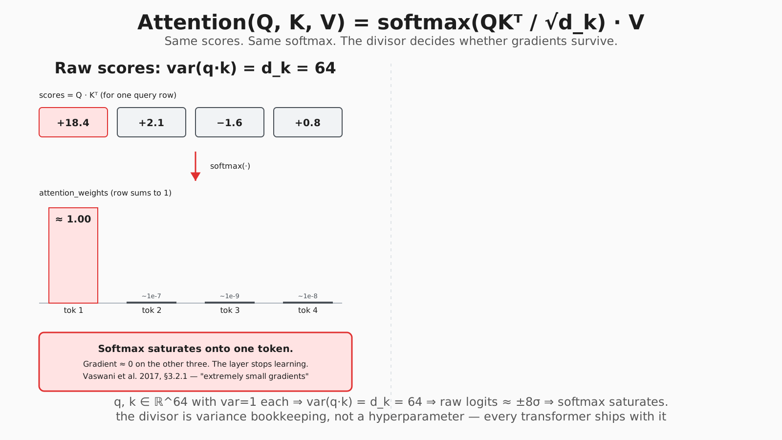
Scaled dot-product attention: the √d_k divisor is variance bookkeeping, not a hyperparameter
Building On Previous Knowledge
The previous chapter ended with one Takeaway: contextual embeddings differ from static embeddings because the surrounding tokens shift the vector. Attention is the mechanism that does the shifting.
A static embedding for bank is one vector. A contextual representation is bank re-mixed with weighted contributions from every other token in the sequence. In river bank that mix leans on river. In savings bank it leans on savings. The mechanism is the same; the inputs differ.
Where most attention tutorials stop: they write softmax(QKᵀ/√d_k)V, label the divisor as “for numerical stability”, and move on. 3Blue1Brown’s transformer videos visualise Q, K, V beautifully but stop short of the variance derivation [3b1b-attention]. The divisor is doing concrete work: without it, the softmax saturates onto one token as d_k grows and the layer’s gradients collapse to zero. This chapter shows the math (Vaswani et al. 2017, §3.2.1, footnote 4 [vaswani2017]), then runs the values through real numbers.
Takeaway: attention is weighted mixing across tokens, and √d_k is not optional — it is the variance correction that keeps softmax differentiable.
What Goes Wrong Without This:
Symptom: Your model truncates long documents and misses important information.
Cause:   You treated context as infinite. Attention is O(n²) in memory.
       128K context doesn't mean you can use 128K without consequences.

Symptom: Model gives inconsistent answers to the same question.
Cause: In long contexts, attention can miss relevant information.
"Lost in the middle" - models attend more to beginning and end.

Symptom: Reasoning fails on complex multi-step problems.
Cause: Attention struggles to carry information across many hops.
Each hop through attention layers is lossy.
Why Attention Matters
Before attention, sequence models used recurrence (RNNs, LSTMs):
Process sequentially:
token_1 → state_1 → token_2 → state_2 → ... → token_n → state_n

Problems:

1. Can't parallelize (each step depends on previous)
2. Long-range dependencies are hard (gradient vanishing)
3. Information bottleneck (fixed-size state)

A 1000-word document must compress through a single state vector.
Attention allows direct connections:
Every token can directly access every other token:

token_1 ←→ token_2 ←→ token_3 ←→ ... ←→ token_n
↑ ↑ ↑ ↑
└───────────┴───────────┴───────────────┘
All pairwise connections

Benefits:

1. Fully parallelizable (all attention computed at once)
2. Direct long-range access (no bottleneck)
3. Dynamic weighting (attend more to relevant tokens)

This is why Transformers replaced RNNs everywhere.
Takeaway: attention’s win over recurrence is parallelism plus direct long-range access — every token reaches every token in one matrix multiply, not through n sequential states.
The Core Idea: Weighted Mixing
Attention is simple at its core:
Input: Sequence of token embeddings [v1, v2, v3, v4]

For each token, compute a new representation by
MIXING all tokens weighted by relevance:

new_v2 = 0.1*v1 + 0.6*v2 + 0.2*v3 + 0.1*v4
↑ ↑ ↑ ↑
weights sum to 1.0 (softmax)

The weights (attention scores) determine how much
each token contributes to the new representation.
For the sentence “The cat sat on the mat”:
When processing "sat":
• High attention to "cat" (subject of sat)
• Medium attention to "mat" (related to sitting)
• Low attention to "the" (less informative)

Result: "sat" embedding now contains information
about WHAT sat (cat) and WHERE (mat).
Takeaway: a token’s post-attention representation is a convex combination of every token’s value vector, weighted by learned relevance — the embedding now carries context, not just identity.
Query, Key, Value
The Q, K, V framework formalizes how attention scores are computed:
┌──────────────────────────────────────────────────────────────────┐
│  INTUITION: Library Metaphor                                     │
├──────────────────────────────────────────────────────────────────┤
│                                                                  │
│  Query (Q): What am I looking for?                               │
│    "I need books about machine learning"                         │
│                                                                  │
│  Key (K):   What does each item contain?                         │
│    Book 1: "Introduction to AI"                                  │
│    Book 2: "Cooking recipes"                                     │
│    Book 3: "Deep Learning fundamentals"                          │
│                                                                  │
│  Value (V): The actual content to retrieve                       │
│    The book's actual contents                                    │
│                                                                  │
│  Match Query against Keys → Weight Values by match quality       │
│                                                                  │
└──────────────────────────────────────────────────────────────────┘
In practice, Q, K, V are linear projections of the input embeddings:
Input embedding: x (dimension d_model)

Q = x @ W_Q # project to query space
K = x @ W_K # project to key space
V = x @ W_V # project to value space

Where W_Q, W_K, W_V are learned weight matrices.

Each token gets its own Q, K, V vectors.
Token i's query asks: "What should I attend to?"
Token j's key advertises: "Here's what I contain"
Token j's value provides: "Here's my information if you want it"
Takeaway: Q, K, V are three separate learned projections of the same input — the model decides per token what to ask, what to advertise, and what to hand over.
Scaled Dot-Product Attention
The standard attention formula:
Attention(Q, K, V) = softmax(QK^T / √d_k) V

Let's break this down:
Step 1: Compute Attention Scores
scores = Q @ K^T

For a sequence of n tokens, each with d_k dimensional Q and K:
Q: (n, d_k)
K: (n, d_k)
K^T: (d_k, n)
Q @ K^T: (n, n) ← attention scores matrix

scores[i][j] = how much token i should attend to token j
Step 2: Scale — Why √d_k Isn’t Optional
This is the step every public attention tutorial under-explains. The divisor is the variance correction that keeps softmax differentiable.
scaled_scores = scores / √d_k

For one query-key pair (q, k) ∈ ℝ^{d_k}:
q·k = Σ q_i · k_i      ← sum of d_k products

If q_i, k_i are independent with mean 0, variance 1:
E[q·k]   = 0
Var(q·k) = d_k         ← variance grows linearly with dimension

For d_k = 64 (Vaswani base model):
std(q·k) ≈ 8
raw logits land at ±8σ → softmax saturates
The original paper states this directly. From Attention Is All You Need §3.2.1, footnote 4 [vaswani2017]:
“To illustrate why the dot products get large, assume that the components of q and k are independent random variables with mean 0 and variance 1. Then their dot product, q·k = Σ q_i k_i, has mean 0 and variance d_k.”
And in §3.2.1 proper:
“We suspect that for large values of d_k, the dot products grow large in magnitude, pushing the softmax function into regions where it has extremely small gradients.”
Concretely: at d_k = 64, raw q·k values land around ±8σ. The softmax of [+18, +2, −2, +1] is roughly [1.0, 1.1e-7, 1.5e-9, 4.2e-8]. Backprop through that softmax — the gradient on three of the four tokens is effectively zero. The layer stops learning.
Divide by √d_k = 8 first and the same logits become [+2.3, +0.26, −0.20, +0.10]. Softmax now yields [0.76, 0.10, 0.06, 0.08] (compute it: e^2.3 ≈ 9.97, e^0.26 ≈ 1.30, e^−0.20 ≈ 0.82, e^0.10 ≈ 1.11; normalise). Every token contributes gradient.
The hero diagram at the top of this chapter shows both rows of numbers side by side.
Takeaway: √d_k is variance bookkeeping. Skip it and softmax collapses onto the single token with the largest raw dot product — at d_k = 64 that happens on essentially every row.
Step 3: Softmax
attention_weights = softmax(scaled_scores)

Softmax converts scores to probabilities:
• All values between 0 and 1
• Each row sums to 1.0
• High scores → high weights, low scores → near zero

Example row: [2.1, 0.5, -1.0, 0.8]
After softmax: [0.65, 0.13, 0.03, 0.19]
↑
Token with score 2.1 gets most attention
Step 4: Weighted Sum
output = attention_weights @ V

Each output vector is a weighted combination of all value vectors:
output_i = Σ (attention_weight[i][j] * V[j])

This is where information actually flows between tokens.
Complete Picture
  Q (n×d_k)        K (n×d_k)
      │                │
      │      ┌─────────┘
      │      │ (transpose)
      ▼      ▼
   ┌────────────┐
   │   MatMul   │  Q @ K^T = (n×n) attention scores
   └─────┬──────┘
         │
         ▼
   ┌────────────┐
   │   Scale    │  divide by √d_k
   └─────┬──────┘
         │
         ▼
   ┌────────────┐
   │  Softmax   │  convert to probabilities (each row)
   └─────┬──────┘
         │
         │      V (n×d_v)
         │         │
         ▼         ▼
   ┌────────────────────┐
   │      MatMul        │  weights @ V = output (n×d_v)
   └─────────┬──────────┘
             │
             ▼
       Output (n×d_v)
Takeaway: scaled dot-product attention is four linear-algebra steps — score, scale, softmax (with optional mask), weighted sum — and the load-bearing one is the divisor.
Multi-Head Attention
One attention pattern isn’t enough. Different relationships need different attention:
"The animal didn't cross the street because it was too tired."

Different questions need different attention patterns:
• Q: What is "it"? → attend "it" to "animal" (coreference)
• Q: What action? → attend verbs to subjects
• Q: What's the reason? → attend "tired" to "didn't cross"

Solution: Multiple attention "heads", each learning different patterns.
Multi-head attention runs h parallel attention operations:
                          Input X
                             │
        ┌──────────┬─────────┼─────────┬──────────┐
        │          │         │         │          │
      ┌─▼─┐      ┌─▼─┐     ┌─▼─┐     ┌─▼─┐      ┌─▼─┐
      │H1 │      │H2 │     │H3 │     │H4 │  ... │Hh │
      │QKV│      │QKV│     │QKV│     │QKV│      │QKV│
      └─┬─┘      └─┬─┘     └─┬─┘     └─┬─┘      └─┬─┘
        │          │         │         │          │
     (n,d/h)    (n,d/h)   (n,d/h)   (n,d/h)    (n,d/h)
        │          │         │         │          │
        └──────────┴─────────┼─────────┴──────────┘
                             │
                       ┌─────▼─────┐
                       │  Concat   │ ← combine heads
                       └─────┬─────┘
                             │
                       ┌─────▼─────┐
                       │    W_O    │ ← project to d_model
                       └─────┬─────┘
                             │
                      Output (n, d_model)
Typical configurations:
┌──────────────────┬───────────────┬───────────────┐
│  Model           │  d_model      │  Heads (h)    │
├──────────────────┼───────────────┼───────────────┤
│  BERT-base       │  768          │  12           │
│  GPT-2           │  768          │  12           │
│  GPT-3 (175B)    │  12288        │  96           │
│  LLaMA 7B        │  4096         │  32           │
└──────────────────┴───────────────┴───────────────┘

Each head has d_k = d_model / h dimensions.
More heads = more diverse attention patterns.
The Vaswani base model uses h = 8 heads with d_model = 512, giving d_k = d_v = 64 per head. The “big” variant uses h = 16 heads with d_model = 1024, keeping d_k = 64 per head [vaswani2017]. Per-head dimensionality stays fixed; the model widens by adding heads, not by enlarging each head.
Why not just one wide head? A single head with d_k = 512 can only learn one weighting pattern per query position — one mixture over keys. Eight 64-dim heads can learn eight mixtures in parallel and concatenate them. The same parameter budget, eight times the expressive bandwidth per layer. Ablation studies on encoder-decoder models reliably show degradation when collapsing to h = 1 for the same d_model, even though parameter count is preserved.
Takeaway: multi-head attention is parallel scaled-dot-product blocks operating on disjoint slices of the embedding — d_k = d_model / h keeps the per-head cost constant as the model widens, and the parallelism is what lets the layer learn distinct relation types simultaneously.
Context Window and Attention
The context window limit exists because attention is O(n²):
For sequence length n:
• Attention matrix: n × n
• Memory: O(n²)
• Compute: O(n²)

┌──────────────────┬───────────────┬───────────────┐
│  Context Length  │   Attention   │    Memory     │
├──────────────────┼───────────────┼───────────────┤
│  1K tokens       │  1M entries   │  ~4 MB        │
│  4K tokens       │  16M entries  │  ~64 MB       │
│  32K tokens      │  1B entries   │  ~4 GB        │
│  128K tokens     │  16B entries  │  ~64 GB       │
└──────────────────┴───────────────┴───────────────┘

This is why long-context models are expensive.
Techniques for Longer Context
1. SPARSE ATTENTION

Instead of n² full attention, attend to subset:
• Local attention: only nearby tokens
• Strided attention: every k-th token
• Random attention: sample positions

BigBird, Longformer use O(n) attention patterns.
Trade: some information paths are blocked.
2. FLASH ATTENTION

Not mathematically different—same result.
But implements attention in a memory-efficient way:
• Never materializes full n×n matrix
• Computes in tiles that fit in GPU SRAM
• 2-4x faster, same memory as single forward pass

This is why modern context windows keep growing.
3. SLIDING WINDOW / RoPE

Combine:
• Rotary Position Embeddings (RoPE) for relative positions
• Sliding window for bounded attention
• Global tokens that always attend everywhere

LLaMA, Mistral use these patterns.
The “Lost in the Middle” Problem
Position in context vs attention received:

Attention │
Score │ ████
│ ████ ████
│ ████████ ████████████
│ ████████████████ ████████████████████████
└──────────────────────────────────────────────
Beginning Middle End

Beginning and end get more attention.
Middle content can be "lost."
Practical impact:
- Put critical information at beginning or end of prompts
- Don’t bury important context in the middle of long documents
- Test your application with information at different positions
Liu et al. 2023 named the U-shape [liu2023]. Chroma’s 2025 Context Rot report measured it across 18 LLMs and showed retrieval accuracy degrades non-monotonically as input grows — sometimes failing on inputs far shorter than the advertised context window [chroma-rot]. A 128K-token model is not 128K-token-effective; benchmark on the lengths your application actually uses.
Takeaway: full attention is O(n²) in memory and compute — a 128K window costs ≈ (128K)² = 16B attention entries per layer per head. Sparse-attention and Flash-Attention implementations buy throughput, not asymptotic relief.
Attention Visualization
What attention patterns look like:
"The cat sat on the mat"

Attention weights (simplified, one head):

         The   cat   sat   on    the   mat
  The   [0.3   0.2   0.1   0.1   0.2   0.1]
  cat   [0.2   0.4   0.2   0.0   0.1   0.1]
  sat   [0.1   0.5   0.2   0.1   0.0   0.1]  ← "sat" attends heavily to "cat"
  on    [0.1   0.1   0.3   0.2   0.1   0.2]
  the   [0.1   0.1   0.1   0.2   0.3   0.2]
  mat   [0.1   0.1   0.2   0.2   0.2   0.2]

Different heads learn different patterns:
• Head 1: Subject-verb relationships
• Head 2: Positional (nearby tokens)
• Head 3: Syntactic structure
Probing studies confirm individual BERT heads specialise. Clark et al. 2019 [clark2019] identified heads in BERT-base that reliably attend to direct objects from their verb, heads that attend across coreference chains (pronoun → antecedent), and heads that latch onto the next or previous token regardless of content. Specialisation emerges from training, not architecture; the architecture only provides h independent slots that the optimiser learns to put to different uses.
This is why pruning attention heads is rarely free — even heads that look redundant on one task are often load-bearing on another. The h dimension is functional capacity, not redundancy.
Takeaway: heads aren’t ensembles of the same thing — each head learns a distinct relation type during training, which is why ablating individual heads degrades different downstream tasks.
Common Pitfalls & Misconceptions
Attention is small, dense, and easy to misread. The errors below show up in production code, tutorials, and interview answers alike.
| Symptom | Cause | Fix |
|---|---|---|
| Loss won’t decrease past epoch 1 on a new transformer block | Forgot to divide by √d_k — softmax collapses onto the largest raw logit, gradient ≈ 0 elsewhere | Apply scores / sqrt(d_k) before softmax; check F.scaled_dot_product_attention is enabled in PyTorch ≥ 2.0 |
| Padded tokens leak into attention weights | Softmax over raw scores treats [PAD] positions as valid keys | Mask before softmax: scores.masked_fill(mask == 0, float('-inf')) — -inf becomes 0 after softmax |
| Causal model peeks at future tokens during training | Decoder used full attention instead of an upper-triangular causal mask | Apply torch.tril mask of shape (n, n) so position i can only attend to positions ≤ i |
| OOM at 32K context on a single GPU | Materialised the full n × n score matrix — at fp16, 32K² is ~2 GB per head per layer | Use Flash Attention via torch.nn.functional.scaled_dot_product_attention (PyTorch ≥ 2.0, [pytorch-sdpa]) or flash-attn package; never materialises the full matrix |
| Q/K/V dimension mismatch error in custom head | Confused d_model with d_k — projecting to d_model per head ignores the d_k = d_model / h split | Project x ∈ ℝ^{d_model} to (h, d_k) via reshape: q.view(batch, n, h, d_k).transpose(1, 2) |
| ”Deterministic” attention output differs across GPUs | Reduction order in matmul is non-deterministic across CUDA kernels; softmax amplifies tiny differences | Accept ~1e-6 fp16 drift as load-bearing; for bit-identity, fall back to fp32 + torch.use_deterministic_algorithms(True) (slow) |
| Multi-head Concat → Linear layer “doesn’t help” | Forgot the final W_O projection — concatenated heads need to be mixed back into d_model space | Add nn.Linear(d_model, d_model) after concat; the paper’s equation calls this W^O and it is learned, not optional |
Takeaway: most attention bugs are masking errors or missing scaling — the architecture is forgiving, the bookkeeping is not.
Code Example
Minimal implementation that mirrors the paper’s equation, written against PyTorch ≥ 2.0. It both implements the formula by hand and shows the production-grade equivalent:
# Tested on torch==2.3.0 (PyTorch ≥ 2.0 required for F.scaled_dot_product_attention)
import math
import torch
import torch.nn.functional as F

def scaled_dot_product_attention(
    Q: torch.Tensor,            # (batch, n, d_k)
    K: torch.Tensor,            # (batch, n, d_k)
    V: torch.Tensor,            # (batch, n, d_v)
    mask: torch.Tensor | None = None,  # broadcast-compatible with (batch, n, n)
) -> torch.Tensor:
    """softmax(Q · Kᵀ / √d_k) · V — Vaswani et al. 2017, §3.2.1."""
    d_k = Q.size(-1)

    # 1. raw attention scores: (batch, n, n)
    scores = torch.matmul(Q, K.transpose(-2, -1))

    # 2. scale by √d_k — the variance correction
    scores = scores / math.sqrt(d_k)

    # 3. optional mask (causal / padding); -inf becomes 0 after softmax
    if mask is not None:
        scores = scores.masked_fill(mask == 0, float("-inf"))

    # 4. softmax → weighted sum of values
    weights = F.softmax(scores, dim=-1)
    return torch.matmul(weights, V)


# Example: batch=2, n=10, d_k=64 (Vaswani base model per-head dimension)
batch_size, seq_len, d_k = 2, 10, 64
Q = torch.randn(batch_size, seq_len, d_k)
K = torch.randn(batch_size, seq_len, d_k)
V = torch.randn(batch_size, seq_len, d_k)

manual = scaled_dot_product_attention(Q, K, V)

# Production code uses the fused kernel (Flash Attention under the hood):
fused = F.scaled_dot_product_attention(Q, K, V)

assert torch.allclose(manual, fused, atol=1e-5)
print(manual.shape)  # torch.Size([2, 10, 64])
Karpathy’s nanoGPT (model.py, CausalSelfAttention.forward) follows the same shape — manual scaling at 1.0 / math.sqrt(k.size(-1)), then prefers F.scaled_dot_product_attention when the runtime is PyTorch ≥ 2.0 [karpathy-nanogpt, pytorch-sdpa].
Verify Your Understanding
Before continuing, you should be able to answer these from memory:
- Why does dividing by
√d_kchange anything? State the variance ofq · kwhenq, k ∈ ℝ^{d_k}have i.i.d. unit-variance components. Predict what softmax does to a row of raw scores atd_k = 64. - What are Q, K, V mechanically? Three learned
Linear(d_model, d_k_or_v)projections of the same input. Explain why splitting Q and K is necessary even though they could share weights in principle. - Single-head vs multi-head with the same total parameters. A model with
d_model = 512, h = 8, d_k = 64has the same parameter count ash = 1, d_k = 512. Why does the paper choose 8 heads? - Lost-in-the-middle and prompt engineering. A 128K-context LLM misses content at the centre of a long document. Name two prompt-restructuring moves that improve recall, and one mechanical reason this happens.
- Memory cost back-of-envelope. Full attention at
n = 32K, fp16materialises ann × nscore matrix. How many GB per head per layer? What does Flash Attention change about that number, and what does it not change?
What’s Next
Attention turned static embeddings into context-aware representations. The next chapter — Attention → Generation — picks up where the last transformer layer ends: how a final hidden state becomes a token, why temperature is not just a knob, and why “deterministic generation” doesn’t exist even at temperature = 0.
References
- [vaswani2017] Vaswani, A. et al. Attention Is All You Need. NeurIPS 2017. arXiv:1706.03762. Source for the scaled dot-product formula, the variance footnote,
d_k = d_model / h = 64for the base model, andh = 16, d_model = 1024for the big model. Cited in §§ Building On Previous Knowledge, Scaled Dot-Product Attention — Step 2: Scale, Multi-Head Attention. - [karpathy-nanogpt] Karpathy, A. nanoGPT. GitHub:
karpathy/nanoGPT,model.pyCausalSelfAttention. Canonical practitioner reference for the PyTorch implementation, including theF.scaled_dot_product_attentionfallback path. Cited in § Code Example. - [3b1b-attention] 3Blue1Brown. Attention in transformers, visually explained. YouTube series, 2024. The clearest visual treatment of Q/K/V as projections; this chapter is complementary in that it does the numerical variance argument the videos leave implicit. Cited in § Building On Previous Knowledge.
- [clark2019] Clark, K. et al. What Does BERT Look At? An Analysis of BERT’s Attention. arXiv:1906.04341. Empirical evidence that individual heads specialise (coreference, direct objects, delimiters) — the basis for the “different heads learn different patterns” claim. Cited in § Attention Visualization.
- [liu2023] Liu, N. F. et al. Lost in the Middle: How Language Models Use Long Contexts. arXiv:2307.03172. Original empirical demonstration of the U-shape attention pattern across position in long contexts. Cited in § Context Window and Attention.
- [chroma-rot] Hong, K., Troynikov, A., Huber, J. Context Rot: How Increasing Input Tokens Impacts LLM Performance. Chroma Technical Report, 2025-07-14. research.trychroma.com/context-rot. Measured retrieval degradation across 18 LLMs as input length grew, including at lengths far below advertised context windows. Cited in § Context Window and Attention.
- [pytorch-sdpa] PyTorch Team.
torch.nn.functional.scaled_dot_product_attention(PyTorch ≥ 2.0). pytorch.org/docs. Fused-kernel attention that dispatches to Flash Attention / memory-efficient kernels. Cited in § Code Example and § Common Pitfalls.